Exploring the Unknown: a Frontier Planner That Learns to Guess

COVER·FRONTIERFLOW·ON-BOARD EXPLORATION, NO NETWORK LINK

The Problem

Put a robot in a building it has never seen. No map, no dropped pins, no human with a joystick. A laser spins on top of it; wheels are underneath. The question is not where to go — it’s how the robot should decide where to go, on its own, until the building is mapped.

The classical answer is called frontier exploration. The idea is old and good: any border between what the robot has seen and what it hasn’t is a frontier, and the frontier most worth visiting is the one that either (a) is close, (b) points the way the robot is already facing, or (c) is likely to lead somewhere useful. “Likely” is where it gets interesting.

We built FrontierFlow, a ROS 2 exploration stack that does the boring parts well and bolts on a small learned model for the less-boring part. 1,312 lines of Python across two nodes, one optional U-Net, a handful of parameters that actually mean something.

Two Nodes, One Map

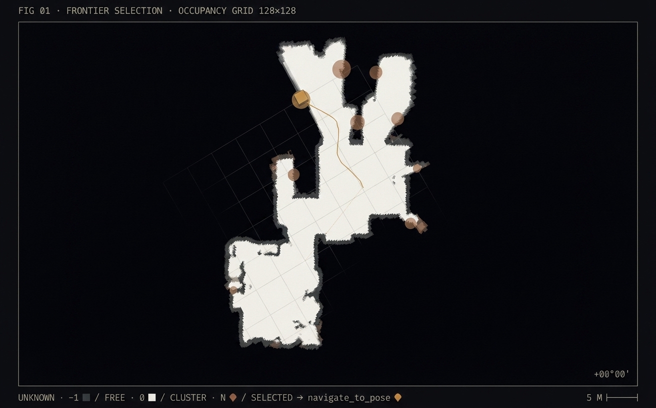
The system is two processes sharing a map.

The first node, frontier_explorer_node, subscribes to the occupancy grid the SLAM stack publishes on /map. It detects frontier cells, clusters them, scores each cluster, and sends the best one as a goal to Nav2’s navigate_to_pose action. When the robot finishes a goal — success or failure — it picks the next one. That’s the whole outer loop.

The second node, map_predictor_node, also subscribes to /map. But it does something odd: it feeds a 128×128 window of the map into a U-Net and guesses what the unknown cells are. Walls or open space. It publishes the result on /predicted_map. The explorer reads that topic, and when it’s deciding between two frontiers, it asks the predictor which one leads somewhere more open.

Neither node touches Nav2’s global costmap. The predictor is optional; if PyTorch is missing or the checkpoint file isn’t there, the system falls back to a pure distance-and-heading heuristic and keeps working.

Detecting Frontiers

A frontier cell is, by convention, a free cell adjacent to an unknown cell. The textbook version is a one-cell check. In practice, that doesn’t work on real SLAM output.

Cartographer — the SLAM we used — inserts a thin border of occupied cells between free and unknown. The border is one or two cells thick depending on scan angle and map resolution. With a one-cell adjacency check, almost no free cell is ever adjacent to an unknown one; they’re separated by this buffer. Frontier detection returns empty, the robot sits still, and you stare at RViz for half an hour before you realise what happened.

The fix is a larger search window. We look within a radius of 2 — a 5×5 box — and call a cell a frontier if any cell in that window is unknown. This happily steps past the one- or two-cell occupied buffer:

# Frontier cell: 0 <= data[idx] < free_thresh and
# at least one cell within 2 cells is UNKNOWN (-1).
# Cartographer places an occupied border between free and
# unknown, so we must look past that 1-2 cell thick wall.
search_offsets = []
for sy in range(-2, 3):
    for sx in range(-2, 3):
        if sx == 0 and sy == 0:
            continue
        search_offsets.append((sx, sy))

frontiers = set()
for y in range(h):
    for x in range(w):
        val = data[y * w + x]
        if val < 0 or val >= free_thresh:
            continue
        for dx, dy in search_offsets:
            nx, ny = x + dx, y + dy
            if 0 <= nx < w and 0 <= ny < h:
                if data[ny * w + nx] == UNKNOWN:
                    frontiers.add(y * w + x)
                    break

The individual cells are then clustered with a standard eight-connected BFS. Anything smaller than min_cluster_cells — 25, by default — is thrown away. Tiny frontier clusters are usually sensor noise: a gap in the scan, one unknown cell surrounded by free ones, a lidar shadow. Chasing them is how you burn a battery going nowhere.

Scoring a Frontier

Given a list of clusters, the explorer picks one. The score is three things multiplied together.

Distance

The base score is (n_cells ^ size_weight) / (dist + 0.1). With size_weight = 0 (our default) it reduces to 1 / dist — the nearest cluster wins. The option to bias toward big clusters is there because on some maps you want it, but we haven’t found a map where we did.

Heading bonus

If the frontier’s centroid is within ±90° of the robot’s current yaw, multiply the score by heading_bonus (1.5). This is not about efficiency. It’s about the robot not looking stupid. Without it, frontiers equidistant left and right of the robot get picked by essentially a coin flip, and the robot spins in place before committing. Three microseconds in code, forty seconds saved on camera.

AI gain

If the U-Net is running, we sample a 7×7 window around the frontier centroid in the predicted map. We count the fraction of cells the model thinks are free. That fraction, in [0, 1], multiplies the base score by 1 + ai_weight × gain:

# Fraction of predicted-free cells in a 7x7 window around
# the centroid. 1.0 = totally open, 0.0 = walls / still unknown.
gx, gy = int(cx), int(cy)
r = 3   # 7x7 window
cnt, free = 0, 0
for dy in range(-r, r + 1):
    for dx in range(-r, r + 1):
        nx, ny = gx + dx, gy + dy
        if 0 <= nx < pw and 0 <= ny < ph:
            v = int(pred_data[ny, nx])
            cnt += 1
            if 0 <= v < free_thresh:
                free += 1
return free / cnt if cnt else 0.0

In practice, the gain term separates two nearby frontiers with similar distances and different futures: one leads into a corner, one leads down a hallway. The corner scores near zero; the hallway scores near one. The hallway wins.

The ProxMaP Assist

The predictor is a small U-Net — four encoder-decoder levels, bilinear upsampling, roughly 1.8M parameters — trained on 2D occupancy-grid completion. Given a partially-known crop of the map, it classifies every cell as free, occupied, or unknown. We take a 128×128 patch centred on the robot’s position, feed it in, and write the predicted free/occupied cells back into the unknown regions of a published /predicted_map.

Two details worth mentioning.

The first is input channels. Older checkpoints take two channels — occupancy plus an unknown mask. Newer ones take three — separate binary channels for known-free, known-occupied, and unknown. We detect which by looking at the weight-tensor shapes in the loaded state dict, at startup, and reshape accordingly. No config flag. The node just does the right thing:

# Accept three checkpoint formats:
#   (a) full torch model object
#   (b) plain state_dict
#   (c) Lightning checkpoint -> dict with 'state_dict'
sd = _extract_state_dict(checkpoint)
in_ch = _infer_in_channels(sd)   # 2 or 3
model = UNet(n_channels=in_ch, n_classes=3, bilinear=True)
model.load_state_dict(sd, strict=False)
model.eval().to(device)

The second is what to do when PyTorch isn’t installed, or the weights file was never copied to the robot, or CUDA is misconfigured and the model takes 6 seconds to run per frame. We have a fallback: a dilation heuristic that looks at each unknown cell, counts free versus occupied neighbours in a radius-3 window, and labels the majority if it passes a 60% threshold. It is not as good as the model. It is also never the reason the robot stops working. That trade is always worth taking.

Inference runs at prediction_rate_hz (1.0 Hz) on a 128×128 patch. On a laptop GPU that’s around 20–50 ms; on the Jetson Nano CPU, closer to 150 ms. The explorer reads the latest /predicted_map whenever it scores frontiers, so nothing blocks on inference.

Preempting Without Thrashing

The most subtle part of the whole system is not the U-Net. It’s knowing when to change your mind.

Here’s the failure mode you’ll hit if you don’t handle this. Robot picks a frontier. Starts driving. Two seconds later, a small bit of map updates, a new frontier appears slightly closer, and its score edges past the current one. The planner cancels the current goal, sends the new one. Two more seconds. Another update. Another cancel. The robot twitches its way through the corridor at half its intended speed because every three seconds it second-guesses itself.

The fix is two numbers and a logbook entry asking why we didn’t do this sooner.

# Only preempt the current goal if BOTH are true:
#   (1) at least preempt_cooldown_sec (60 s) has elapsed
#       since we sent the current goal, AND
#   (2) the new frontier's score is more than
#       preempt_score_ratio (2.0) times the current score.
cooldown_ok = (now - goal_sent_at) >= preempt_cooldown_sec
ratio_ok    = new_score >= current_score * preempt_score_ratio

if cooldown_ok and ratio_ok:
    self._cancel_current_goal()
    self._send_goal(best_frontier)

Sixty seconds of cooldown. Two-times-better threshold. Both have to clear. With this rule the robot commits, drives, arrives, and only reconsiders when something meaningfully new shows up — a big unexplored wing, an obvious shortcut. The twitching stops.

The Parameters That Matter

You could tune a lot of knobs. In practice, five of them matter.

There is also a blacklist. Goals that Nav2 rejects or fails get added to it for 60 seconds; goals the robot actually reaches get added for 120 seconds. The longer blacklist on success is there so the robot doesn’t immediately re-propose the cell it just stood on as a new frontier the moment the map flickers around it.¹

What We’d Change

Three things, in the order we’d do them.

1. A reachability check before sending the goal.

Right now we rely on Nav2 to reject unreachable goals. That round-trip takes a couple of seconds we don’t have to burn. A quick look-up against the global costmap would filter obvious losers up front. The reason we didn’t do this is architectural tidiness — we liked the explorer not knowing about costmaps — but the tidiness isn’t worth a tenth of the cost.

2. A smarter predictor input.

The U-Net sees the map. It doesn’t see the lidar, the recent scans, or the direction the robot last moved in. Feeding even a scan-derived occupancy hint as an extra channel would, we suspect, sharpen predictions near the edge of the map — which is exactly where we use them.

3. Multi-robot coordination.

Running two robots in the same building with the same planner produces two robots that both pick the same closest frontier and argue about it with their navigation stacks. A shared blacklist and a cheap auction would fix it. It is, to us, the single most obviously missing thing — and the reason we wrote this one to be a single file per robot, clean inputs, no global state.

Three features. Three microamps of effort. That’s the next post.²