The Mission
A small quadcopter over a wooded valley. Somewhere below, a person who is not supposed to be there — lost, or exactly where they shouldn’t be. The camera sees everything and nothing; it produces a stream of frames far faster than a human can scan them, and it is attached to a flight controller that would very much like to know, in real time, whether there is a human in the field of view.
This is the kind of task that attracts the wrong answer. "Upload frames to a server and run a big model" is the wrong answer because the drone is five kilometres from the nearest cell tower. "Run a big model on the drone" is the wrong answer because the drone’s compute budget is a Raspberry Pi 4 and a thermal envelope that does not forgive 85% CPU for an hour.
The right answer is a small model. Smaller than feels comfortable. Small enough to run on a Pi 4 CPU, alongside flight telemetry and a camera pipeline, and still keep up with the frame rate.
We trained a YOLOv8n variant on three classes — smoke, fire, human — merged from two public datasets, then quantised it to INT8 and exported it to TFLite. This is the writeup.
Two Datasets, One Label Space
There is no single dataset in the world that covers what we needed. D-Fire has smoke and fire boxes, drawn on aerial and street-level imagery, labelled as classes 0 and 1. SARD — Search and Rescue Drone — has humans in outdoor, top-down, drone-perspective imagery, labelled as class 0. Both are YOLO-format; neither has the other’s labels.
The merge is a trick older than deep learning and will outlive it: remap label indices so the two datasets agree, then concatenate. We rewrote every SARD label file from class 0 (human) to class 2, kept D-Fire’s 0 (smoke) and 1 (fire) unchanged, and wrote a single merged_data.yaml pointing at both sets of images:
train:
  - /kaggle/input/.../smoke-fire/data/train/images
  - /kaggle/working/sard/train/images
val:
  - /kaggle/input/.../smoke-fire/data/val/images
  - /kaggle/working/sard/valid/images
nc: 3
names: ['smoke', 'fire', 'human']
What you end up with is 18,163 training images — 14,122 from D-Fire, 4,041 from SARD — and a label space where the model learns all three classes simultaneously from the beginning, rather than trying to merge two pretrained heads at the end. The ratio is roughly 3:1 in D-Fire’s favour, which means "human" is the minority class in raw counts. The per-class mAP numbers later in the post suggest this didn’t hurt as much as we feared.
One implementation wrinkle worth mentioning: 26 images across the two datasets had read errors during the Kaggle training run — files on a read-only filesystem that Ultralytics couldn’t open. The trainer logged each one and skipped it. Not a problem at this scale; on a smaller dataset it would be.
Training, as Boringly as Possible
YOLOv8n is the smallest model in the v8 family. 3.01 million parameters, 8.2 GFLOPs, 130 layers. Starting from the COCO-pretrained checkpoint, we transferred 319 of 355 weight tensors; the rest are the head, which is re-initialised because we have three classes, not eighty.
Training hyperparameters were chosen to be unsurprising:
- Optimiser: AdamW, learning rate 0.001, weight decay 0.0005, cosine schedule, 3-epoch warmup
- Batch size: 32 (single Tesla T4 at 14.9 GB)
- Image size: 640×640 during training, 320×320 at export
- Epochs: 100 with a patience of 20 (never triggered)
- Augmentation: mosaic 1.0, mixup 0.1, hsv, random flips in both axes, 45° rotations, 0.5× scale jitter. Mosaic turned off for the last 10 epochs — standard trick to let the model see clean single-frame samples before freezing
The whole run took 6.04 hours of wall time on the T4. Long enough for the learning-rate schedule to matter; short enough that a second attempt with different hyperparameters doesn’t bankrupt the project.
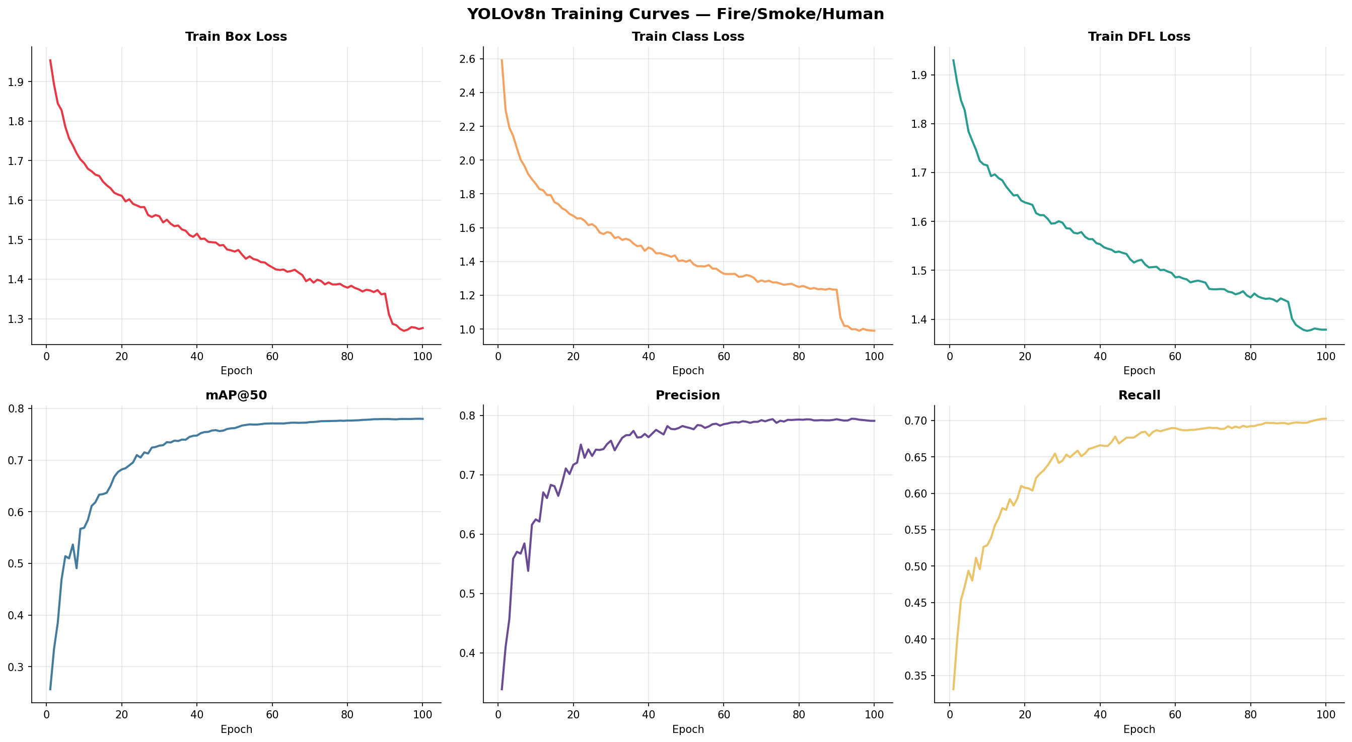
Nothing surprising in the curves. Losses fall, mAP rises, both settle. The close-mosaic transition at epoch 90 shows up as a small uptick on validation — the model briefly does better on the clean-augmentation frames before re-equilibrating. We shipped the best weights from that range.
The Numbers
Final validation metrics on the 4,238-image held-out set, measured in the standard COCO way:
| Metric | Value |
|---|---|
| mAP@50 | 0.781 |
| mAP@50-95 | 0.430 |
| Precision | 0.792 |
| Recall | 0.701 |
The more interesting number is per-class. Averaging papers over the signal:
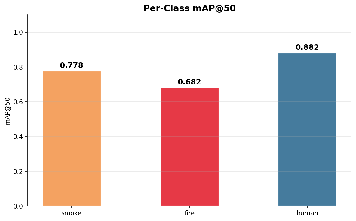
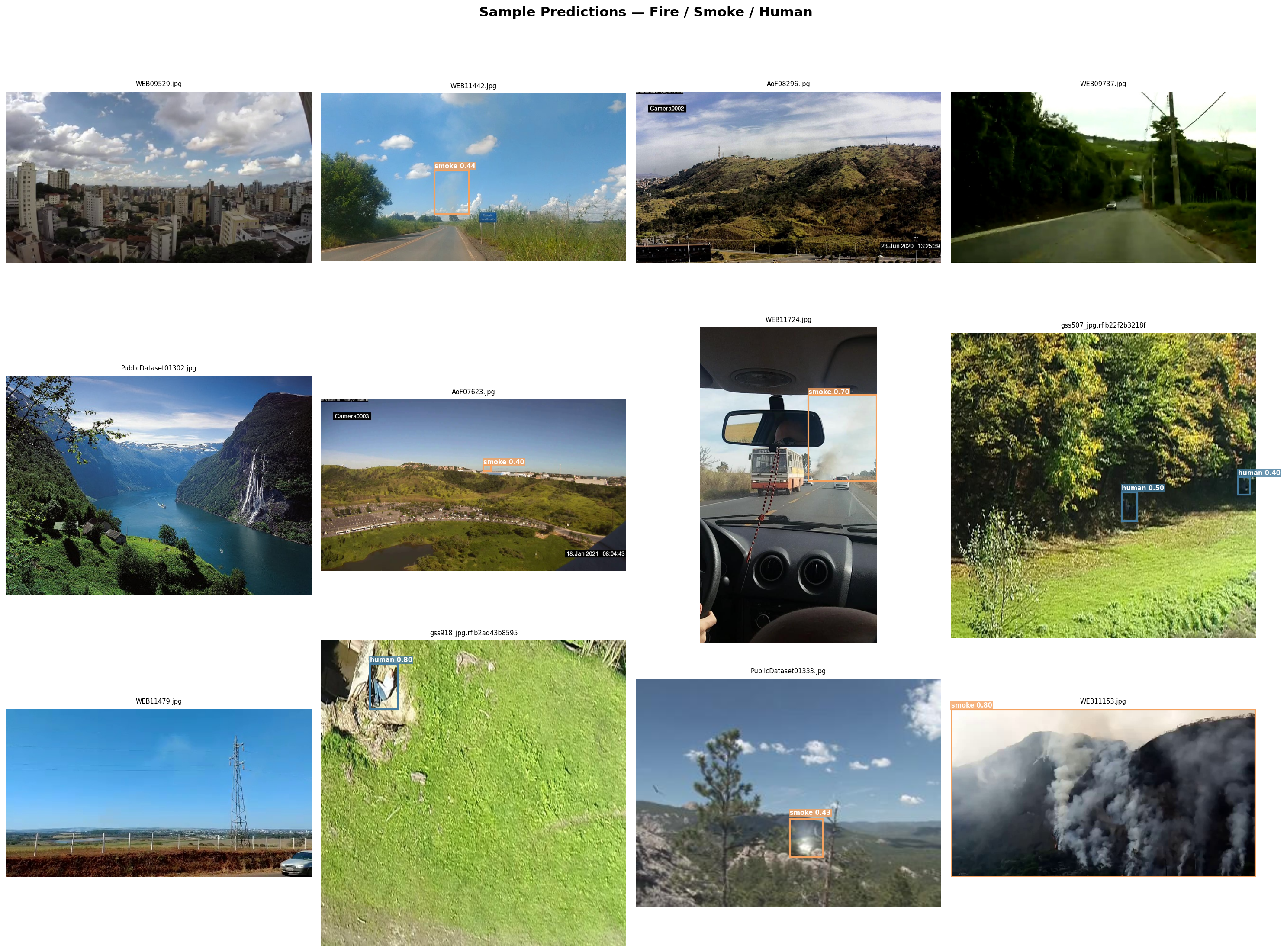
Three observations, all of them useful.
Human is the easiest class. mAP@50 of 0.88 and recall of 0.83. This surprised us at first — human is the minority class by training count. What it actually says is that the SARD images are consistent in framing (top-down, outdoor, human roughly centre-frame, clean background) while D-Fire is wildly varied (CCTV frames, webcam stills, outdoor landscapes, fire-brigade footage). Uniform data, even less of it, makes for better-calibrated detectors.
Fire is the hardest class. 0.68 at mAP@50. Looking at the failure cases, the pattern is predictable: small fires overlap visually with reflections, sunlight on glass, vehicle tail-lights, tungsten-coloured signage. The model is right to be uncertain about those, but it costs us precision.
Smoke is in the middle. 0.78. Smoke is an amorphous class — the bounding-box premise is already a bit of a lie for it — and the model does about as well as it can. The D-Fire dataset has a mix of thin smoke plumes and heavy industrial clouds, and the model handles both.
Shrinking It for a Pi
A 640×640 float32 YOLOv8n that mAPs at 0.78 is worth nothing on a Pi 4 if it takes 800 milliseconds per frame. The export is where the project becomes useful.
Two things happened at once. We dropped the input resolution from 640 to 320, and we quantised the weights to INT8. These are not free operations — both hurt accuracy a little. We measured how much.
| Format | Input | Size | Notes |
|---|---|---|---|
PyTorch best.pt | 640 | 6.2 MB | Training checkpoint, FP32 |
best_int8.tflite | 320 | 3.0 MB | INT8, Pi 4 target, preferred |
best_ncnn_model/ | 320 | 11.6 MB | Backup path when TFLite is ornery on ARM |
best.onnx | 320 | 11.6 MB | Intermediate for other targets |
The 3 MB TFLite INT8 file is the one that ships. Drop in resolution cuts FLOPs by a factor of four; INT8 quantisation replaces 32-bit multiplies with 8-bit ones and is a dramatic real-world speedup on the Pi 4’s NEON SIMD lanes. Together, per-frame inference on the Pi sits comfortably under 100 ms, leaving headroom for camera I/O and the flight stack.
For the INT8 calibration step, TFLite needs representative input data — you cannot pick a quantisation scale for weights and activations without seeing the distribution of real activations. We pointed it at the validation set. The export runs each image through the model, records activation ranges, picks per-layer scales and zero-points, and bakes them into the flatbuffer. Roughly 1,000 images, 90 seconds, done.
NCNN is the backup. It ships as two files — a .param graph description and a .bin weight blob — and sometimes beats TFLite on ARM CPUs by a surprising margin. We export it alongside so there is no rebuild cycle if TFLite turns out to be slow on the specific Pi revision in the drone.
What Went Wrong First
Before we had this result, we had three failed results. Worth naming them.
1. We trained without the mosaic close-out.
The first 100-epoch run kept mosaic augmentation on for every epoch. Validation mAP climbed, then plateaued oddly — a class of errors where the model clearly understands the task but refuses to commit to tight boxes. Turning mosaic off for the last ten epochs fixed it. The model spends those final epochs seeing clean, single-image frames, and it tightens up its predictions accordingly. Cost: one additional training cycle and a cup of coffee.
2. We tried imgsz=320 end-to-end.
The thinking was: the target device runs at 320, train at 320 so there’s no train-inference mismatch. The resulting model mAP was about four points lower. YOLO’s augmentation pipeline — especially mosaic, which composites four images into one — genuinely benefits from the extra resolution during training. The right recipe is train at 640, export at 320.
3. We didn’t remap the SARD labels at first.
If you leave SARD’s human class as 0, and then merge with D-Fire where 0 is smoke, you get a model that is remarkably confident that people are smoke. It’s funny for about ten minutes. The remap script — four lines of Python — is the most important four lines in the whole project.1
Parameters
The handful of knobs that materially change the outcome:
| Name | Default | What it changes |
|---|---|---|
imgsz (train) | 640 | Driver of model capacity. Don’t go below this unless you must. |
imgsz (export) | 320 | Driver of latency. Halving this quarters the compute. |
close_mosaic | 10 | Last N epochs with mosaic disabled. Matters more than people say. |
mixup | 0.1 | Mild. Zero it out if you’re overfitting badly; raise it cautiously. |
lr0 | 0.001 | AdamW comfort zone. Stick close. |
int8 | true | The difference between "runs on a Pi" and "doesn’t". |
What We’d Change
Three directions.
1. A fourth class: "human, likely in distress".
Drones in search-and-rescue miss the interesting case frequently because detection treats all humans identically. A second label — distinguishing a walking person from someone lying prone or waving — would be a much better operational signal. This is a labelling problem, not a model problem, and it’s where the next month of data work would go.
2. A NEON-tuned NMS kernel.
A non-trivial slice of Pi-side inference time is non-maximum suppression — the step that collapses hundreds of overlapping boxes into a few clean ones. The default implementation does not use NEON. A hand-rolled version would shave another few milliseconds off the per-frame budget.
3. Temporal smoothing.
Right now each frame is classified independently. A simple IOU-tracker over the last three frames would let us trade a millisecond of compute for much calmer, less flickery detections on the downlink. It would also give us, for free, basic tracking output that the flight controller can act on — "the person has been at bearing 34° for 2.1 seconds" is actionable in a way that 15 independent detections per second is not.2
- The label remap is the kind of bug that looks like a modelling problem for two hours before anyone thinks to look at the labels. Whenever a model is performing implausibly well or implausibly badly, open a terminal and
head -5on the first label file. - The astute reader will notice that most of the ideas in this section are "do the obvious next thing". That is the case study; it is rarely otherwise.